Here’s a simple dataset - just two variables that we’ll call \( x \) and \( y \).

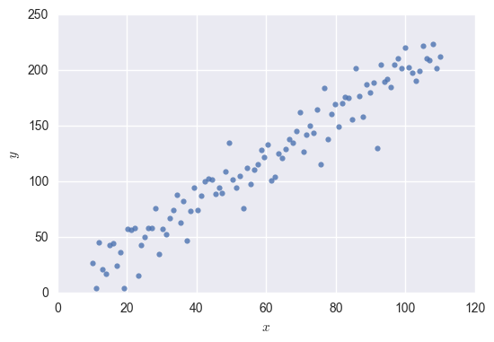
It looks like \( x \) and \( y \) are related! Let’s say we want to use \( x \) to predict \( y \). We can use regression to fit a function to the data. Here is our function plotted over the data:

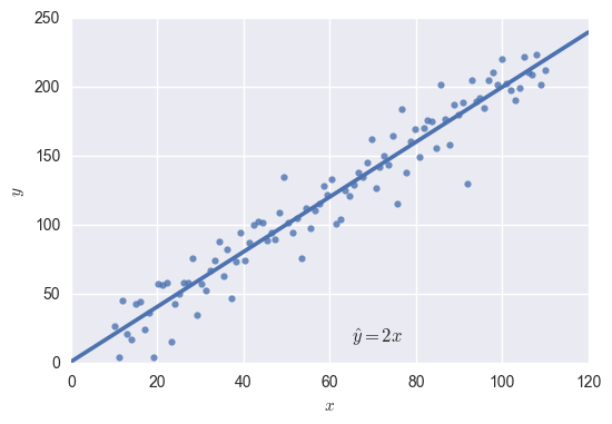
A pretty good fit! This was a simple regression problem, because for every unit increase in \( x \), \( y \) also increases some proportionate amount. The equation for the above line is \( \hat y=2x \), so we know that for every unit increase in \( x \), \( y \) increases by about 2.

What do we do when fitting the data isn’t so easy, such as when our data looks like this?

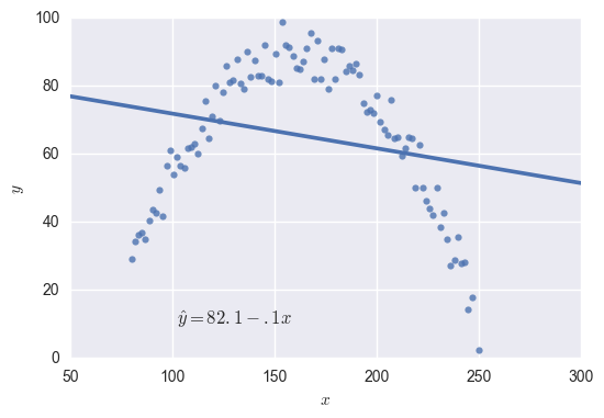
The equation for this function is \( \hat y=81.6-.1x \), and it doesn’t fit the data very well. Rather than \( y \) varying as a function of \( x \), it looks like \( y \) varies as a function of \( x^2 \). This means we want to look for a function of the form \( y=\beta_0+\beta_1x+\beta_2x^2 \). Our regression software will take care of finding the best \( \beta \) values; we just need to give it an \( x \) variable as well as an \( x^2 \) variable to work with.

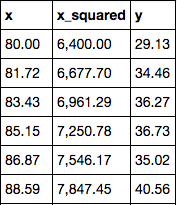
So I square my \( x \) values, and now I have data that looks like this:

I run regression to predict \( y \) in terms of these two other variables, and I get:

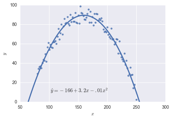
That worked pretty well!

The principle here is to try and understand how my \( y \) variable varies as a function of my \( x \) variables, and then transform my \( x \)’s to match that function.

Sometimes, having an understanding of the subject matter that you’re dealing with can help you do this. Take a look at one more example using some made-up data:

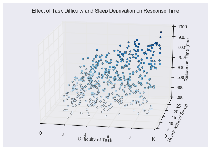
Imagine this data comes from a psychology experiment where participants complete tasks of varying difficulty after being kept awake for varying numbers of hours. The experimenter measures how participant response time (in milliseconds) on the tasks changes as a function of task difficulty and sleep deprivation. (Note that we have to visualize this in 3-D, because we now have three variables.)

If we wanted to make predictions based on this data, we would try to predict response time (our \( y \) variable) using task difficulty and sleep deprivation (our two \( x \) variables).

Let’s again use regression to fit a function to this data without doing any kind of transformation beforehand. Here’s what we get:

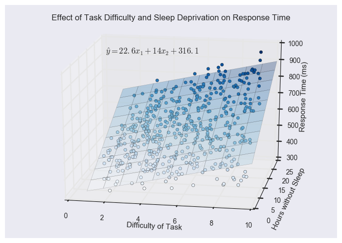
The equation for this function is \( \hat y=22.6x_1+14x_2+316.1 \), and as you were probably expecting, it isn’t a good fit. The bottom right corner of the plane is too high, whereas the top right corner is too low to fit the data correctly.

An experienced researcher might guess that there is an interaction between your \( x \) variables. This would mean that, say, a difficult task increases response time, but it increases response time even more when you’re sleep deprived. Mathematically, an interaction would look something like \( y=\beta_0+\beta_1x_1+\beta_2x_2+\beta_3x_1x_2 \). Notice the last term of the equation has \( x_1 \) and \( x_2 \) multiplied by each other.

Let’s add an interaction term to our data, then, and see how it fits. As before, this is as simple as creating a new variable that is the product of \( x_1 \) and \( x_2 \). When we run regression to predict \( y \) in terms of \( x_1 \), \( x_2 \), and \( x_1x_2 \), we get:

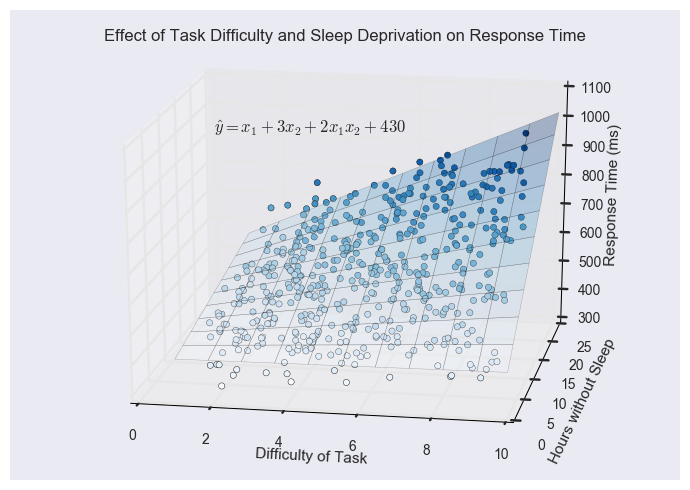
This is a good fit! The function now bends to show the interaction between task difficulty and sleep deprivation. Look at the bottom of the plot - for someone who has had plenty of sleep, as task difficulty increases, response time only increases a little bit. But at the top of the plot we can see that for someone who is sleep deprived, as task difficulty increases, response time increases a lot.

Conclusion

These are just a few common transformations you might need to do to your data to fit a regression. It’s also common to do a \( \log \) transformation, or create higher-order polynomial variables like \( x^3 \) or \( x^4 \).

I hope this helps build your intuition about using regression to fit a function to your data!